
Fundamentals of Statistics
- Hussam Omari
- 12 فبراير 2023
- 13 دقيقة قراءة

Table of Contents
What is Statistics?
Statistics is a branch of applied mathematics. It can be defined as the science of creating, developing, and applying techniques by which uncertainty of inductive inferences may be evaluated. Statistics is a field of study concerned with collection, organization, summarizing and analysis of data and drawing inferences about population data when only a part of the data (data sample) is obtained.
There are two main branches of statistics; descriptive and inferential. Descriptive statistics is a branch of statistics that is concerned with summarizing and describing data. The goal of descriptive statistics is to provide a concise summary of key features of a dataset, such as the sample size, mean, median, mode, variance, and standard deviation. These measures can be used to get a sense of the distribution of the data, as well as any outliers or unusual observations.
There are many different techniques used in descriptive statistics, including frequency distributions, histograms, box plots, and scatter plots. These techniques can be used to visualize the data and help identify patterns or trends. Additionally, measures of central tendency, such as the mean and median, can be used to describe the "typical" value in a dataset, while measures of dispersion, such as the variance and standard deviation, can be used to describe the spread of the data.
Inferential statistics is another branch of statistics that involves makes inferences or estimates about a population based on a sample of data. They consists of methods for drawing and measuring the reliability of conclusions about a population based on information obtained from a sample of the population; such as t-test, ANOVA, correlation and regression.
Population and Sample
In statistics, a population is the entire group of individuals or objects that you are interested in studying or making inferences about. A sample, on the other hand, is a subset of the population that you collect data from (Figure 1).
The main difference between a population and a sample is that a population includes all the individuals or objects of interest, while a sample is a smaller subset of the population.
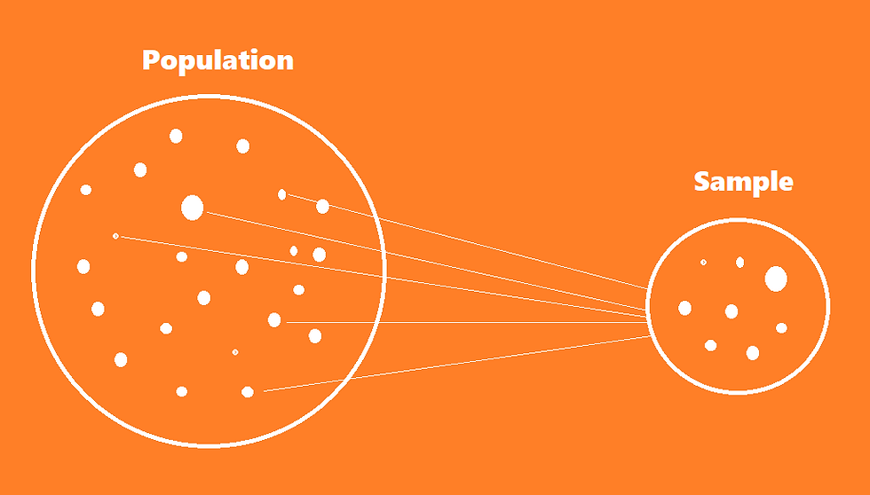
Figure 1: A visual representation of selecting a Sample from a Population
Often, collecting data on the entire population can be time-consuming, expensive and impractical, therefore researchers use samples to make inferences and draw conclusions about populations.
For example, let's say we want to study the income of all adults in a country, the population would be all adults in that country. Usually, we do not have the resources to collect data on every individual of a population. Instead, we collect data on a random sample of individuals and use descriptive and inferential statistics to obtain estimations and make inferences about the population of all individuals based on our sample.
For this purpose, we can use statistical sampling techniques such as Random Sampling, Clustered Sampling, Systematic Sampling, Stratified Sampling, etc.
Parameter and Statistic
Statistics and parameters are fixed values that describes or summarizes a characteristic of a population. A parameter is a value that describes or summarize a characteristic of a population and is usually unknown (e.g. the mean height of all people on earth), while a statistic is a value that describes a characteristic of a sample taken from the population (e.g., mean height of people sampled from several countries).
In other words, a parameter is a value that is fixed and true for an entire population, while a statistic is a value that is estimated from a sample and used to infer information about the population. For example, the mean income of a population is a parameter, while the mean income of a sample of people is a statistic.
In order to estimate a population parameter, we take a sample from the population and calculate a statistic (e.g. mean, variance and standard deviation) from that sample. The statistic is then used as an estimate of the population parameter. However, it is important to note that there is always a margin of error (sampling error) between the statistic and the parameter.
Variables in Statistics
In statistics, a variable refers to a characteristic or attribute that can take on different values for different individuals or observations. In research, a variable is any quality or characteristic in a research investigation that has two or more possible values.
For example, variables in studies of how well seeds germinate might include amounts of sun and water, kinds of soil and fertilizer, genetic makeup of the seeds, speed of germination, and hardiness of the resulting plants. Variables in studies of how effectively children learn in classrooms might include instructional methods used; teachers’ educational backgrounds, emotional warmth, and beliefs about classroom discipline; and children’s existing abilities and personality characteristics, prior learning experiences, reading skills, study strategies, and achievement test scores.
Types of Variables
In statistics, variables are classified into two main categories: categorical and numerical (Figure 2). The type of variable will determine which type of statistical analysis can be performed on the data, and can affect the interpretation of results.
Categorical variables (qualitative variables) represent characteristics that can be divided into groups or categories. Examples include gender, race, and religious affiliation.
Numerical variables represent quantities or measurements (numerically valued variables). They can be either discrete or continuous. Discrete variables can only take on specific, distinct values such as integers, while continuous variables can take on any value within a certain range, such as weight or height. Continuous variables are also known as quantitative variables.
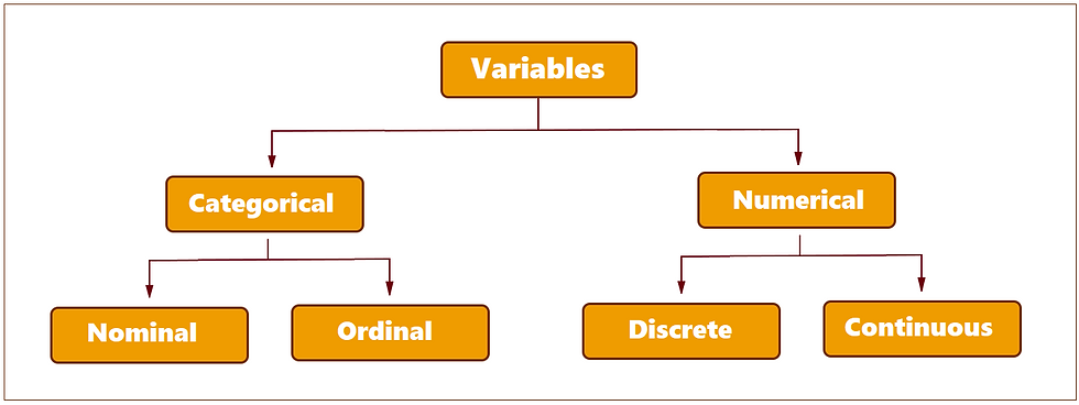
Figure 2: Main types of variables in statistics
Dependent vs. Independent Variables
An independent variable is a possible cause of something else or that is used to predict the value of another variable (dependent variable). In many experimental studies, a variable can also be a factor that is manipulated or controlled to investigate its effect or relationship to one or more dependent variables.

A dependent variable is a variable that is affected by the independent variable and its status depends to some degree on the status of the independent variable. Note that dependent variables are the ones that are measured in an experiment.
For example, a study conducted to investigate the effect of temperature (15, 20, and 25 °C) and on plant height and chlorophyll content. In this study, the independent variable is temperature and this variable has three levels (15, 20, and 25 °C); whereas, the dependent variables are plant height and chlorophyll content.
Other Types Variables
There are other types of variables in research such as mediating, moderating, and extraneous and confounding variable.
A mediating variable - also known as intervening variable - is a variable that explains the relationship between an independent variable and a dependent variable. It mediates the relationship between the independent and dependent variables.

A moderating variable is a variable that does not intervene between the independent and dependent variables, but influences the nature and strength of their cause-and-effect relationship.

Extraneous variables are not of primary interest in a study but they may affect the relationship between the independent and dependent variables, but are not part of the experimental design. They are "controlled" and measured in order to eliminate their effect on the results.
A confounding variable is an extraneous variable that is "not controlled" and may affect the relationship between the independent and dependent variables in an unknown way.
The Sampling Distribution of a Normally Distributed Variable
Data distribution refers to the way that values are spread out among a dataset. The data distribution is a key concept to understanding the statistical inference. To get better understanding of data distribution concept, we first need to understand the frequency distribution and the sampling distribution.
The data distribution is closely related to the frequency distribution. A frequency distribution is the number of times (frequency) of each value or range of values occurs in a dataset. It is a way to summarize and represent the distribution of a set of continuous or categorical data. A frequency distribution can be represented in various forms like tables and histograms.
A histogram is a graphical representation of a frequency distribution that uses rectangles to show the number of observations within a given interval. a histogram is a useful representation for identifying patterns and outliers in the data, as well as for making probability calculations.
As previously mentioned, when we want to study a population, we draw a sample randomly from that population. Once the sample is selected or collected, various statistical methods can be used to make inferences about the population based on the sample data (i.e., sampling distribution).
A sampling distribution is the probability distribution of a sample statistic (e.g. mean, proportion). It is a theoretical concept that describes how the sample statistic would vary if we repeated the process of sampling many times from the same population.
For instance, by using the sampling distribution (Figure 3), we can estimate the mean or proportion of a population, test hypotheses about population parameters, and construct intervals that are likely to contain the true population parameter with a certain level of confidence (usually 99 or 95%).
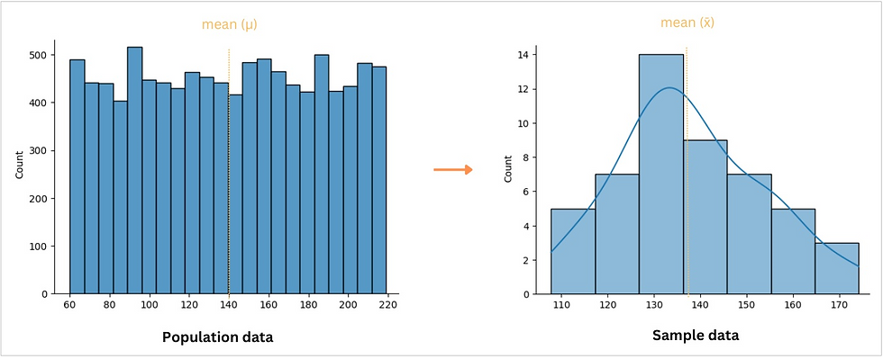
Figure 3: A histogram visualization for a population and sample distribution
Based on the central limit theorem, you don not need to sample a population repeatedly to know the shape of the sampling distribution. The parameters of the sampling distribution are determined by the parameters of the population.
The Central Limit Theorem
The central limit theorem (CLT) states that if you take sufficiently large samples from a population, the samples’ means will be normally distributed, even if the population is not normally distributed.
The CLT is a fundamental principle in statistics because it allows us to use normal distribution methods to make inferences about a population even if the sample data drawn from the population is not normally distributed.
It is important to note that the CLT holds when the sample size is sufficiently large, usually larger than 30. Also the CLT applies when the samples are independent and randomly drawn, and when the underlying population distribution is not normal but it is finite.
The Normal Distribution
A variable or dataset is said to be "normally distributed", if its distribution has the shape of a normal curve. The normal curve is a symmetric bell-shaped curve with a single peak, and the majority of the values fall within one standard deviation (𝜎) of the mean; this means that the majority of the values cluster around the mean (average) value and the number of values decreases as you move away from the mean in either direction.
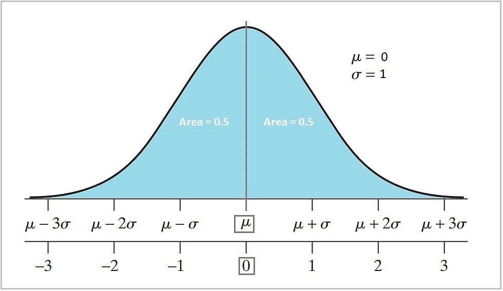
Figure 4: The normal curve and its properties
In real world, a data distribution is unlikely to have exactly the shape of a normal curve. If the distribution is shaped almost like a normal curve, we usually say that the variable is an approximately normally distributed.
The normal distribution (also known as Gaussian distribution) is very important. It is often used in statistics and other fields to model and describe real-world data because its shape is defined by the mean (equals 0) and standard deviation (equals 1), which makes it easy to work with mathematically by transforming real-world data to make it approximately normally distributed, a process known as standardizing the data.
One common method for doing this is to convert the data to standard scores, also known as z-scores. By converting the data to z-scores, we can standardize the data so that it has a mean of 0 and a standard deviation of 1, which makes it approximately normally distributed.
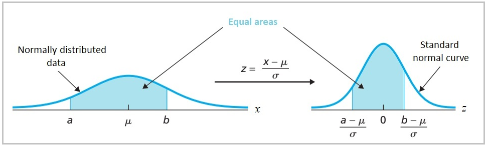
Figure 5: Illustration and formula for transforming raw scores into a z-scores.
However, it is important to note that not all data sets can be made perfectly normally distributed by standardization. Some data sets, such as those with a large number of outliers, may not be able to be made normally distributed through standardization or any other method. In these cases, it may be necessary to use other methods, such as nonparametric statistical tests, that do not rely on the assumption of normality.
Also, it is important to note that standardizing the data does not make it normal but it makes the data follows a standard normal distribution which is a normal distribution with mean 0 and standard deviation 1.
The Empirical Rule
The empirical rule, also known as the 68-95-99.7 rule or the three-sigma rule, is a statistical rule that describes the distribution of data around the mean for a normal distribution.
If the distribution of the data set is approximately bell-shaped; that are not too skewed, we can apply the empirical rule, which implies the following:
Approximately 68% of the data values lie within 1 standard deviation (𝜎) on each side of the mean.
Approximately 95% of the data values lie within 2 standard deviations on each side of the mean.
Approximately 99% of the data values lie within 3 standard deviations on each side of the mean.
This means that if the data is approximately normally distributed, then almost all of the data (99.7%) will fall within three standard deviations of the mean (Figure 6).
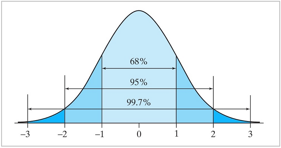
Figure 6: The normal curve and its properties
The empirical rule is a useful tool for understanding the spread of data in a normal distribution and for identifying outliers in a data set.
Hypothesis Testing
A statistical hypothesis testing is the process of expressing an assumption to help us decide whether our data sufficiently support our hypothesis. It helps us to decide whether the data is consistent with the experimental hypothesis or not.
We formulate the hypothesis before test calculations such as t-test. This hypothesis is simply a prediction statement also known as experimental or research hypothesis which is a statement about the relationship or difference between groups that we want to test. This prediction statement is based on the experimental hypothesis, which is a claim or assumption about the population. In other words, we translate our experimental hypothesis into statistical hypothesis.
The statistical hypothesis test includes two statements or hypotheses; the null hypothesis and alternative hypothesis.
The null hypothesis (H0) is the the hypothesis to be tested. This hypothesis assumes that there is no difference or no relationship between groups — the group means are statistically equal. Hence we can express the null hypothesis as

This means that any differences or similarities observed in the sample data are likely due to chance and not due to any underlying relationship or difference in the population and the results of the hypothesis test do not provide enough evidence to reject the null hypothesis in favor of the alternative hypothesis.
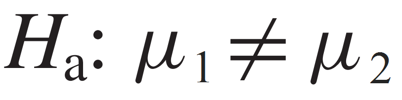
The alternative hypothesis (Ha) is the alternative to the null hypothesis. This hypothesis assumes that there is a difference between groups. Three choices are possible for the alternative hypothesis:
If the primary concern is deciding whether a group mean (μ1) is statistically not equal to another mean (μ2); two-tailed test, then we express the alternative hypothesis as:
If the primary concern is deciding whether a group mean is statistically less than another mean (lift-tailed test), we express the alternative hypothesis as:

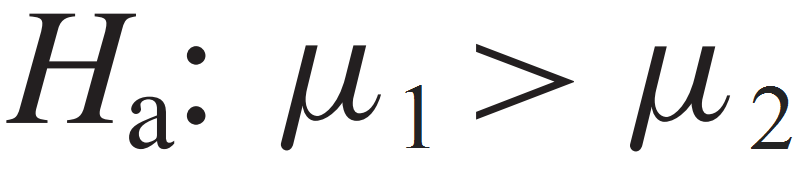
If the primary concern is deciding whether a group mean is statistically higher than another mean (right-tailed test), we express the alternative hypothesis as:
Example: Suppose a researcher want to investigate the effectiveness of a new medication (Nuvacin) for treating a certain medical condition. The experimental hypothesis for this study might be that Nuvacin is more effective than a famous current medication. The null hypothesis would be that there is no difference in effectiveness between the new medication and the current medication. Note that the medication Nuvacin is an imaginary name.
To test this hypothesis, the researcher would randomly assign patients with the same medical condition to either receive Nuvacin (group 1) or the current medication (group 2). The researcher would then collect data on the patients' health outcomes (scores) and use statistical tests, such as a t-test, to compare the effectiveness of the two medications (Figure 7).
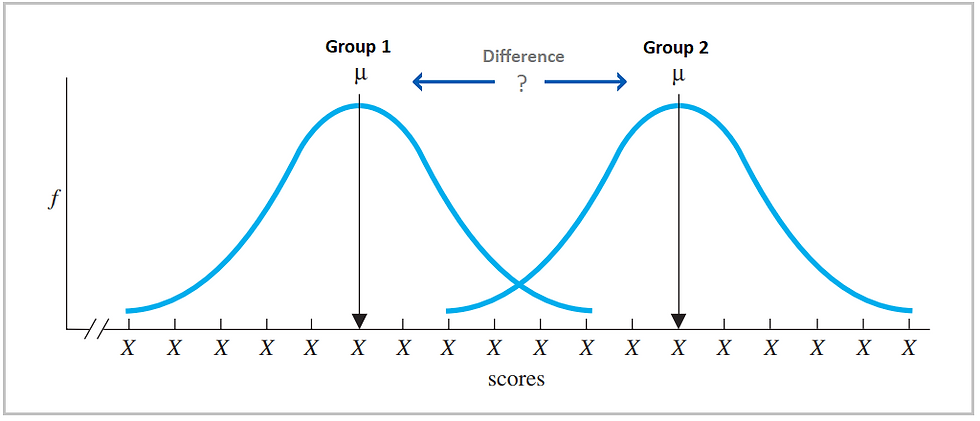
Figure 7: A representation of the basic logic of the statistical difference between groups
If the results do NOT indicate a statistically significant difference, the researcher would fail to reject the null hypothesis (H0), and conclude that there is not enough evidence to support the research hypothesis and there is no difference in effectiveness between the two medications.
If the results of the hypothesis test indicate that there is a statistically significant difference in effectiveness between the new medication (Nuvacin) and the current medication, the researcher would reject the null hypothesis in favor of the alternative hypothesis (H1). This indicates that there is a significant difference between the two medications and since the group who received Nuvacin has higher mean value, then Nuvacin is more effective than the current medication.
This is an example of a simple experimental design, but there are many variations of it depending on the research question and the complexity of the study.
Making Errors in Hypothesis Testing
Statistical hypothesis testing is all a matter of probabilities and statistical inferences are based on incomplete information (a sample of data); hence, there is always a risk of making an error and there is always the chance that we could make either a Type I or Type II error.
In hypothesis testing, a type I error occurs when the null hypothesis (H0) is REJECTED when it is actually TRUE. This is also known as a false positive or alpha error. The typical significant levels (α) in most researches is 0.05, which means that there is a 5% chance of making a type I error.
A type II error occurs when the null hypothesis is NOT REJECTED when it is actually FALSE (Figure 8). This is also known as a false negative or beta error. The probability of a type II error is dependent on the sample size, effect size, and power of the test.
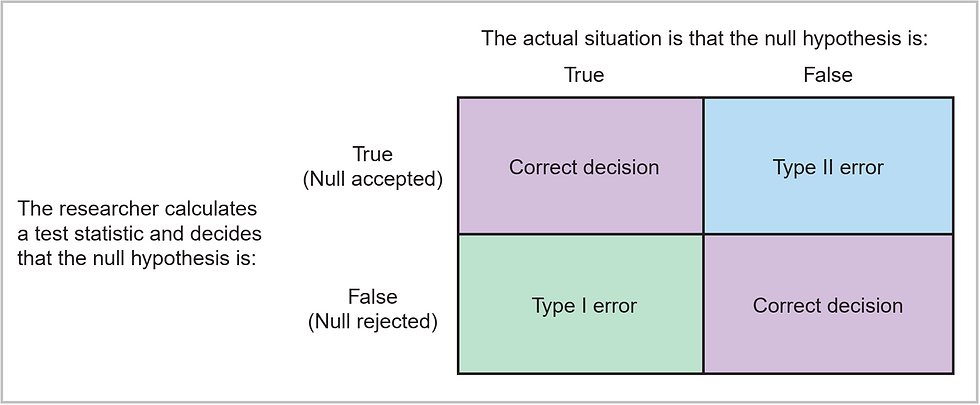
Figure 8: Outcomes of statistical decision-making. Source: Polit & Beck (2010)
There is a trade-off between Type I and Type II errors: Whenever you decrease the risk of making one, you increase the risk of making the other. Therefore, researchers use various techniques to control the probability of making these errors, such as setting a significance level (α) for the test, say from 0.05 to 0.01, also using larger sample sizes.
However, it is not always possible to completely eliminate the risk of making an error. Therefore, when researchers analyze the data obtained from the groups under study to get the results tables, they focus on Type II error rather than Type I error because in many cases, the consequences of a Type II error can be more serious in some fields, such as medical research, than Type I error. Thus, it is important to control for Type II error when designing and interpreting experimental studies.
Types of Statistical Tests
There are two main types of statistical test; parametric and nonparametric tests. Parametric tests typically use continuous data (e.g., weight, height, temperature, time). These data types are often used in parametric tests because they meet the assumptions of normality and equal variances that parametric tests rely on. Some examples of parametric tests include:
Student t-test: used to compare the means of two groups
ANOVA: used to compare the means of three or more groups.
Correlation: used to measure the strength of a linear relationship between two variables.
Linear Regression: used to model and examining the relationship between variables and making predictions.
Nonparametric tests are also known as distribution-free tests and often used when the assumptions of parametric tests, such as normality and equal variances, are not met. Nonparametric tests can be used with both continuous and categorical data. Some examples of nonparametric tests include:
Chi-square test: used to compare observed results with expected results.
Wilcoxon rank-sum test: used to compare the medians of two groups.
Mann-Whitney test: used to compare the medians of two groups.
Kruskal-Wallis test: used to compare the medians of three or more groups
Spearman's rank correlation: used to measure the strength of a non-linear relationship between two variables.
References
Mendenhall, W. M., & Sincich, T. L. (2016). Statistics for Engineering and the Sciences Student Solutions Manual (6th ed.). USA: Taylor & Francis Group, LLC.
Heiman, G. W. (2011). Basic Statistics for the Behavioral Sciences (6th ed.). USA: Cengage Learning.
Samuels, M. L., Witmer, J. A., & Schaffner, A. (2012). Statistics for the Life Sciences (4th ed.): Pearson Education, Inc.
Weiss, N. A., & Weiss, C. A. (2012). Introductory Statistics (9th ed.): Pearson Education, Inc.
Polit, D. F., & Beck, C. T. (2010). Essentials of nursing research: Appraising evidence for nursing practice (7th ed.): Lippincott Williams & Wilkins.
Leedy, P. D., & Ormrod, J. E. (2015). Practical research: Planning and design. USA: Pearson Education.


تعليقات