
Two-way Analysis of Variance (ANOVA)
- Hussam Omari
- 12 فبراير 2023
- 5 دقيقة قراءة


In the previous article, we explained the One-way Analysis of Variance (one-way ANOVA) which is an inferential statistics used to determine if there is a significant difference between the means of more than two groups. There are different versions of ANOVA are used depending on the design of a study.
The one-way ANOVA is used when only one independent variable is tested in the experiment, whereas a two-way ANOVA is used with two independent variables. In other words, we use the two-way ANOVA when we want to know how two independent variables (factors), in combination, affect a dependent variable.
One-way vs Two-way ANOVA
To clarify the one-way ANOVA, suppose, for example, we conducted a study about spraying three concentrations of a growth stimulant (2, 4, and 6 ml/l) on corn plants. Later, we measured the height of each plant sprayed with specific concentration of the three. The plant height in this experiment is considered the dependent variable because the plants height values are affected by the the growth stimulant concentrations, whereas the growth stimulant itself is considered the independent variable which is also known as "factor".
In addition, each concentration is considered a factor level and in this example we have 3 factor levels (3 concentrations), therefore we have 3 plant groups; each group received similar concentration (Figure 1).
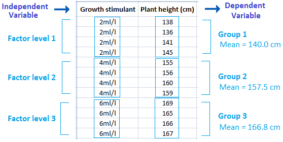
Figure 1: A data with one factor (independent variable) designed for one-way ANOVA
In two-way ANOVA, we have two independent variables that both manipulate e dependent variable. Suppose we conducted a study about spraying three concentrations of a growth stimulant (2, 4, and 6 ml/l) on corn plants, and in the same time these plants were grown in three different type of soils (sand, silt, and clay). The measurement taken at the end of the study was plant height.
In this experiment, we have one dependent variable (plant height) and two independent variables (two factors or treatments); the growth stimulant and the type of soil (Figure 2).

Figure 2: Data with two factors (independent variables) designed for two-way ANOVA
Post Hoc Test
As we mentioned previously, ANOVA is used to determine if a significant difference between the means of three groups or more is existed or not. However, F statistic in ANOVA doesn't tell us which of the groups significantly differs from the other groups, therefore we need further tests that help us to detect which means are significantly differ from other means' groups; this kind of test are known as post hoc tests.
Post hoc tests are like t-tests in which we compare all possible pairs of means from a factor or factors, one pair at a time, to determine which means differ significantly. The most common post hoc tests are the following:
Fisher's Least Significant Difference (LSD)
Duncan's new multiple range test (MRT)
Dunn's Multiple Comparison Test.
Holm-Bonferroni Procedure.
Scheffé's Method.
Tukey's test
Comprehensive Example
Let's bring and analyze the growth stimulant data of the previously mentioned example (Figure 2). The study was conducted to measure the effect of a growth stimulant on corn plants. The plants were grown in three different type of soils (sand, silt, and clay) and sprayed with three concentrations of a growth stimulant (2, 4, and 6ml/l). At the end of the experiment, we measured the height of each plant that were sprayed with specific concentration of the three.
The ANOVA and Post Hoc Test Results
The ANOVA results, presented in Figure 3, are obtained using SAS software. Notice that the p-value of the probability value of F (significance value) of the overall ANOVA test is less than the critical value (Pr < 0.05). In addition, the F value of the main effect (soil) , the main effect (growth stimulant; concentrations), and the interaction effect of both (soil type × growth stimulant) are significant. These results indicate that at least one of the groups' mean under study are significantly differ from other groups' means.
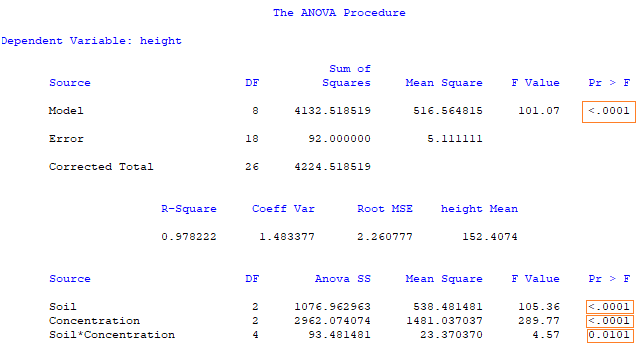
Figure 3: The ANOVA tables of growth stimulant data
Note that the main effect, in this context, is the effect of just one of the independent variables (one factor) on the dependent variable, while the interaction effect represents the combined effects of two factors or more on the dependent measure.
Since the F values are significant, we can now compare the mean values using post-hoc test such as LSD test, as shown in Figure 4 and 5. Notice that each plants group' mean is denoted with a subscription letter (A, B, or C), and since each mean has different letter, this indicates a significant difference between the mean and the other means. Also, the highest mean values is denoted with A letter, while the lesser mean values are denoted with C and so on. In summary, if two means or more were denoted with same letter, these means are statistically equal and there is no significant difference among them.
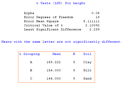
Figure 4: Post hoc test for the main effect of soil type on corn plants
The results presented in Figure 4 indicated that plants' group grown in clayey and silty soil showed significantly higher plants height mean compared to plant grown in Sandy soil. The highest plant height mean was observed in plants group grown in clayey soil compared to all other plants groups.
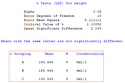
Figure 5: Post hoc test for the main effect of growth stimulant on corn plants
The results presented in Figure 5 indicated that plants' group sprayed with 6ml/l and 4ml/l concentration of plant growth stimulation showed significantly higher plants height mean compared to the plants sprayed with 2ml/l. The highest plant height mean was observed in plants group prayed with 6ml/l concentration compared to all other groups.
Concerning the interaction effect, we used SAS version 9.0 to analyze the data and this version lacks to the subscription letters that show significant difference between the means, therefore we did it manually as shown in Figure 6.

Figure 6: Table and bar chart representation of the interaction effect of soil type and growth stimulant concentration on plants height.
Results presented in Figure 6 showed that corn plants sprayed with 6 and 4ml/l growth stimulant and grown in clayey soil, followed by plants prayed with 6ml/l and grown in silt soil, scored the highest height mean compared to all other plants groups. However, the lowest plant height was observed in plants sprayed with 2ml/l and grown in sandy soil.
References
Mendenhall, W. M., & Sincich, T. L. (2016). Statistics for Engineering and the Sciences Student Solutions Manual (6th ed.). USA: Taylor & Francis Group, LLC.
Heiman, G. W. (2011). Basic Statistics for the Behavioral Sciences (6th ed.). USA: Cengage Learning.
Samuels, M. L., Witmer, J. A., & Schaffner, A. (2012). Statistics for the Life Sciences (4th ed.): Pearson Education, Inc.
Weiss, N. A., & Weiss, C. A. (2012). Introductory Statistics (9th ed.): Pearson Education, Inc.


تعليقات