
Linear Correlation & Regression
- Hussam Omari
- Apr 10, 2022
- 5 min read

Updated: Nov 24, 2022

Linear regression and correlation are closely related subjects in which both are commonly used methods for examining the relationship between quantitative variables and for making predictions. Both requires scores from two variables (x and y). Also, both techniques are based on fitting a straight line to the data.
In this Article, we introduce methods for describing relationships and association between two numerical variables and for assessing the strength of a relationship using linear regression and correlation coefficient.
Correlation Coefficient
In previous articles, we discussed Descriptive Statistics - Essentials and Interpretation. Descriptive statistics are simply describing what is or what the data shows. They summarize the characteristics of a data set and enable us to present the data in a more meaningful way. One of the remaining types of descriptive statistic for us to discuss is used to summarize relationships, and it is called the correlation coefficient. There are several types of correlation coefficient, but the most popular is the linear correlation coefficient (r) which is also called the Pearson's product moment correlation coefficient and is commonly used with linear regression.
The linear correlation coefficient is a numerical assessment of the strength of relationship between the x and y values in a bivariate dataset consisting of (x, y) pairs. In other words, the correlation coefficient tells us two major things; how strong the relationship between two variables, and if they are statistically related, do they move in same direction or opposite directions.
The term linear means “straight line,” and a linear relationship forms a pattern that follows one straight line. This is because in a linear relationship, as the X scores increase, the Y scores tend to change in only one direction (increase or decrease).
The value of the correlation coefficient (r) ranges between -1 and 1. A positive value of r suggests that the variables are positively linearly correlated, meaning that y tends to increase linearly as x increases, with the tendency being greater the closer that r is to 1. A negative value of r suggests that the variables are negatively linearly correlated, meaning that y tends to decrease linearly as x increases, with the tendency being greater the closer that r is to −1.
To graphically demonstrate the meaning of the linear correlation coefficient, we present various degrees of linear correlation in Figure 1.

Figure1: Basic degrees of linear correlation. Source: Introductory Statistics, Neil A. Weiss, 9th edition, 2012.
Note that if r is close to ±1, the data points are clustered closely about the regression line. If r value is farther from ±1, the data points are more widely scattered about the regression line. If r is near 0, the data points are essentially scattered about a horizontal line indicating at most a weak linear relationship between the variables.
Example: Linear Correlation
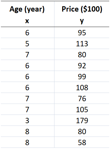
Suppose we have a dataset contains age and price of 11 Sedan cars (Table 1) and we wish to see whether there is a relationship between the age and price of these cars. In other words, we want to know that as the cars age (x) increases, does the cars price (y) increase or decrease?
Table 1: Age and price of Sedan cars
We can easily obtain the linear correlation between age and price in this dataset using several statistical analysis software and programming languages such as SPSS, SAS, Minitab, Python and R. However, in this tutorial we used SPSS to generate correlation table as shown in Table 2.
Table 2: SPSS results - correlation table
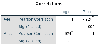
As shown in Table 2, the linear correlation coefficient (r) is -0.924 and it is statistically significant (Sig. < 0.05). This suggests a strong negative linear correlation between age and price of Sedan cars which indicates that as Sedan age increases, there is a strong tendency for price to decrease, and the data points are clustered closely about the regression line.
Since the linear correlation coefficient (r = -0.924) is close to -1 and highly significant (sig. < 0.05), this indicates that when we perform a linear regression analysis, the regression formula will be extremely useful for making predictions, which we discuss in the next section.
The Linear Regression
It is very important to understand the linear regression because it is used to predict the unknown Y scores based on the X scores, and this prediction is used in many research studies, especially in correlational studies.
Regression procedures center around drawing a linear regression line which is the line that best fits a set of data points according to the least-squares criterion. The least-squares criterion is that the line that best fits a set of data points is the one having the smallest possible sum of squared errors that keep all deviations (errors or residuals) minimized as small as it can be (Figure 2).
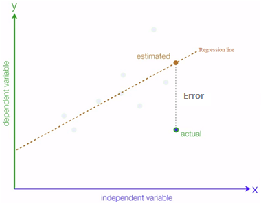
Figure 2: Illustration of linear regression line that best fits a set of data points. The Errors are the vertical distances from the estimated regression line to each data point (actual). Note that x is the independent variable, and y is the dependent variable.
The basic idea of linear regression is to determine the slop (b1) and y-intercept (b0). The b1 and b0 values enables us to formulate the linear regression equation (Figure 3) that is used to predict the y-value when x-value equals a specific value within the dataset. The b1 measures the steepness of the line (slope); more precisely, b1 indicates how much the y-value changes when the x-value increases by 1 unit.
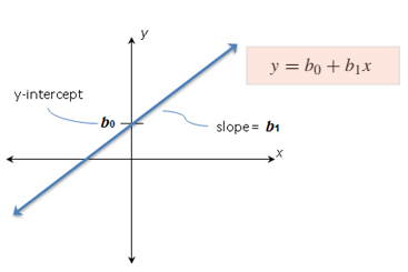
Figure 3: Illustration of slope, y-intercept and linear regression equation.
Note: Always compute the linear correlation coefficient (r) first to determine whether a relationship exists or not. If the correlation coefficient is not 0 and passes the inferential test, then perform linear regression to further summarize the relationship.
Example: Linear Regression
In this example, we demonstrate the linear regression by returning to the data of the previous example [age and price for a sample of Sedan cars]. In the previous example we determined the correlation coefficient (r). The r value was -0.924 and it is statistically significant (Sig. < 0.05) and close to -1. This suggests a strong negative linear correlation between age and price of Sedan cars. Therefore, we can precede and perform the linear regression for this data. When you perform the linear regression through SPSS, the outcomes are several tables. Usually we concern about two tables; the ANOVA and the coefficients table as shown in Figure 4.
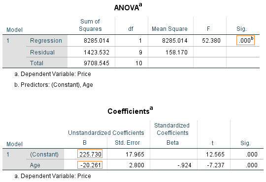
Figure 4: The linear regression results tables for Sedan cars' age and price dataset
The ANOVA table, which reports how well the regression equation fits the data, indicates that the regression model predicts the dependent variable significantly well. Look at the "Regression" row and go to the "Sig." column. The Sig value is less than 0.05 which indicates that the overall regression model significantly predicts the outcome variable ( it is a good fit for the data).
The Coefficients table provides us with the necessary information to predict price from age, we can use the values in the "B" column which represent the y-intercept (225.73) and the slope (-20.26) to represent the regression equation as shown in Figure 5.
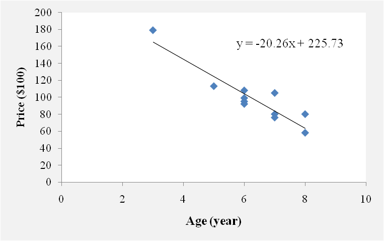
Figure 5: Graphical representation of Sedan cars' age and price data points with the regression line and equation
By substituting the x value in the regression equation, we can predict the y-value when x-value equals a specific value. Suppose we wish to estimate the y-value (Sedan car price) when x-value (Sedan car age) equals 9 years. We can do that by using the formula presented in Figure 5 as follows:
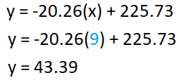
Based on the regression equation of Sedan cars' age and price dataset, we can say that when the age of a Sedan car is 9 years, the price is around $4339.
References
Mendenhall, W. M., & Sincich, T. L. (2016). Statistics for Engineering and the Sciences Student Solutions Manual (6th ed.). USA: Taylor & Francis Group, LLC.
Peck, R., Olsen, C., & Devore, J. L. (2012). Introduction to Statistics and Data Analysis (4th ed.). Boston, USA: Cengage Learning.
Samuels, M. L., Witmer, J. A., & Schaffner, A. (2012). Statistics for the Life Sciences (4th ed.): Pearson Education, Inc.
Weiss, N. A., & Weiss, C. A. (2012). Introductory Statistics (9th ed.): Pearson Education, Inc.
Heiman, G. W. (2011). Basic Statistics for the Behavioral Sciences (6th ed.). USA: Cengage Learning.


Comments