
Multiple Linear Regression
- Hussam Omari
- Jun 4, 2022
- 4 min read

Updated: Jan 23, 2023

In the previous article, we explained the linear correlation and simple linear regression which are commonly used methods for examining the relationship between quantitative variables and for making predictions. Both requires scores from two variables (x and y). Also, both techniques are based on fitting a straight line to the data.
The term linear means “straight line,” and a linear relationship forms a pattern that follows one straight line. This is because in a linear relationship, as the X scores increase, the Y scores tend to change in only one direction; increase or decrease (Figure 1).
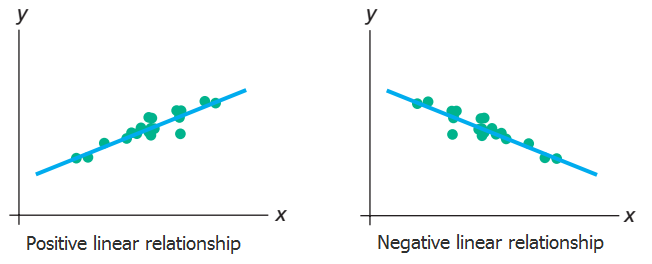
Figure 1: In a positive linear relationship, as x increases, y also increases. In a negative linear relationship, as x increases, y decreases.
Simple linear regression is used to predict the unknown Y scores based on the X scores. In other words, we predict the dependent variable (Y) values based on only one independent variable (factor) values. However, in multiple linear regression, we use two or more independent variables to predict the unknown Y values. Therefore, multiple linear regression is considered an extension of the simple linear regression.
In simple linear regression, there is just one Y variable and one X variable (factor). Whereas, in multiple linear regression, there is one Y variable and two or more X variables (independents).
Before you perform multiple linear regression, your data should meet the following assumptions:
The data needs to show linear relationship between the dependent and independent variables.
The independent variables (factors) are not highly correlated with each other.
No significant outliers, high leverage points or highly influential points.
Your data needs to show homoscedasticity, which is where the variances along the line of best fit remain similar as you move along the line.
You need to check that the residuals (errors) are approximately normally distributed.
Example
The following data, presented in Table 1, represents the profit margin (Y) of savings and loan companies in a given year, the net revenues in that year (X1), and number of savings and loan branches offices (X2). Our goal is to know whether there is enough evidence, at the α = 0.05 level of significance, to conclude that at least one of the predictors (X1 and X2) is useful for predicting profit margin; therefore the model us useful. Also, to predict the profit margin for a bank with 3.5 net revenues and 6500 branches.
Table 1: Profit margin data for savings and loan banks.
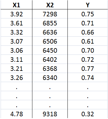
The Y variable represents the profit margin of savings and loan companies in a given year. The X1 represents the net revenues in that year. The X2 represents the number of savings and loan branches offices (X2).
In this example, we can notice that the dependent variable is the profit margin (Y), and the independent variables are the net revenues in that year (X1), and number of savings and loan branches offices (X2).
When you perform the linear regression through SPSS, the outcomes are several tables. Usually we concern about three tables; Model Summary, the ANOVA and the Coefficients table as shown in Figure 2 and 3.
Results presented in the Model Summary table showed that the coefficient of multiple determination (R-squared) is 0.865; therefore, about 86.5% of the variation in the profit margin is explained by net revenues and number of branches for the savings and loan banks. The regression equation appears to be very useful for making predictions since the value of R-squared is close to 1.
Results presented in the ANOVA table revealed that the Sig. value (p-value) is ≤ 0.05, therefore we can conclude that there exists enough evidence to conclude that at least one of the predictors is useful for predicting profit margin; therefore the model us useful.
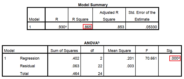
Figure 2: The Multiple linear regression SPSS results; Model Summary and ANOVA tables.
Results presented in Figure 3 showed the Coefficients table which provides us with the necessary information to predict the profit margin based on the net revenues in that year (X1), and number of savings and loan branches offices (X2).
The Coefficients table revealed that the Sig. value (p-value) is ≤ 0.05, therefore we can conclude that there exists enough evidence to conclude that the slope of the net revenue variable and number of savings and loan branches offices are useful as a predictors of profit margin of savings and loan banks.

Figure 3: The Multiple linear regression SPSS results; Model Summary and ANOVA tables.
Since the Coefficients table provides us with the necessary information to predict, we can predict the profit margin (Y) for a bank with 3.5 net revenues (X1) and 6500 branches (X2) by substituting the X1 and X2 value in the following regression equation:
y = 1.564 + (0.237)X1 + (-0.000249)X2
y = 1.564 + (0.237)3.5 + (-0.000249)6500
y = 0.775
We can conclude that when the net revenue is 3.5 and branches are 6500, the point estimate of the profit margin is 0.775.
Multiple vs. Multivariate Linear Regression
As previously mentioned that multiple linear regression is a statistical method that is used to model the relationship between a dependent variable and one or more independent variables. The model is called multiple because it uses multiple independent variables to predict the value of the dependent variable.
On the other hand, multivariate linear regression is similar to multiple linear regression, but it uses multiple dependent variables instead of just one. The model is called multivariate because it uses multiple dependent variables to predict the values of the independent variables.
In summary, multiple linear regression has multiple independent variables and one dependent variable, while multivariate linear regression has multiple independent variables and multiple dependent variables.
References
Mendenhall, W. M., & Sincich, T. L. (2016). Statistics for Engineering and the Sciences Student Solutions Manual (6th ed.). USA: Taylor & Francis Group, LLC.
Peck, R., Olsen, C., & Devore, J. L. (2012). Introduction to Statistics and Data Analysis (4th ed.). Boston, USA: Cengage Learning.
Samuels, M. L., Witmer, J. A., & Schaffner, A. (2012). Statistics for the Life Sciences (4th ed.): Pearson Education, Inc.
Weiss, N. A., & Weiss, C. A. (2012). Introductory Statistics (9th ed.): Pearson Education, Inc.
Heiman, G. W. (2011). Basic Statistics for the Behavioral Sciences (6th ed.). USA: Cengage Learning.


Comments