Data Analysis with Python: Top Countries in Publication Production

Table of Contents

What is Python?

What is SCImago?

Pre-Requests

The Analysis Process

Conclusions

What is Python?

Python is an open-source programming language and one of the most popular and rapidly growing high-level programming languages worldwide. It is used for different proposes including Software development, machine learning, and data science including data analysis and visualization. In this article, we use Python (version 3.10.6) to analyze and visualize SCImago Country Rank data. The Python codes will be written as simple as possible, so you can understand each step easily.

What is SCImago?

The SCImago Journal & Country Rank (SJR) is a publicly available portal that includes the journals and country scientific indicators, such as number of scientific publications, number of citations and H-index, developed from the information contained in the Scopus database (Elsevier).

The Data sheets (2017-2021) was obtained from the SJR website and then combined in one Excel sheet. Before reading any further, it is recommended to download the following Excel file and open the whole data to see its arrangement and structure.

scimagojr country rank 2017-2021

.xlsx

Download XLSX • 82KB

Pre-Requests

For this entire analysis, it is recommended to use Jupyter Notebook. You can easily get Jupyter by downloading and installing Anaconda for free from their website. Personally, I run Jupyter Notebook in Visual Studio Code. For more information, see the following articles:

• Python Basics: Installation, Syntax, Variables and Operations

• Jupyter Notebooks in VS Code

You also need to install the following Python libraries:

• openpyxl

• pandas

• numpy

• scipy

• seaborn

• matplotlib

We explained these libraries usage and installation in the previous article "Top Python Libraries for Data Analysis".

However, after installing Python on your machine, you can install any of these libraries by typing the following command in your Command Prompt:

pip install package_name

To install pandas library, for example, open the Windows Command Prompt (Figure 1) from the Start Menu, and then type the following command:

pip install pandas

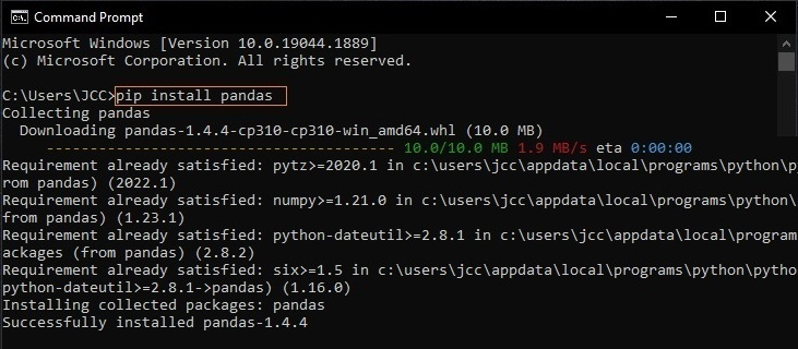
Figure 1: installing Pandas package

The Analysis Process

Defining the Questions

The first step in any data analysis process is to define the questions that we need to answer through data analysis. This step is essential because the data analysis results should answer these questions to attain our objective(s) and to extract insights from the data.

We are going to analyze the SCImago data to answer the following questions:

• What is the total number of publications by year (2017-2021)?

• What are the top regions in number of publications?

• What are the top 5 countries in number of publications?

• How strong the correlation between number of publications and H-index?

Importing Libraries and DataFrame

After downloading the Excel data file (.xlsx) and opening the Jupyter Notebook, you need to import the libraries as well as the data (DataFrame) as shown in Figure 2.

It is recommended to save the Jupyter file and the data file in the same directory (same folder), thus you do not need to type the full directory of the data file within the pandas code.

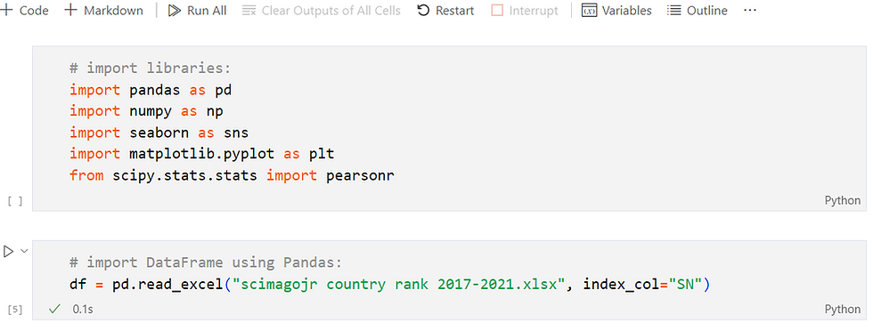
Figure 2: Importing libraries and Data file

Understanding Our DataFrame

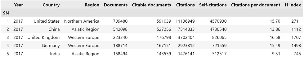
After importing the data, we need first to explore our data variables and data shape. We can start doing so by checking the head of the DataFrame by using the head() method to view the columns names (variables) and the first rows of the DataFrame, as follows:

# Return the first 5 rows
df.head()

Output:

Similarly, you can also use .tail() method to view the last rows of the DataFrame.

From the output above, you can see that SCImago Country Rank data contain 9 different variables (columns names). The variables that we will use to answer our questions are the following:

1. Year: The year of publication

2. Country: The country of the publication

3. Region: The region of the publication

4. Documents: The number of publications

5. H index: A metric used to measure the publications impact

The next step is getting the shape of our DataFrame. In other words, we need to know how many rows and columns that the DataFrame contains. To do so, run the following code:

# Return the dimensionality of the DataFrame:
df.shape

Output:

(1164, 9)

From the output above, we know that our DataFrame contains 1164 rows and 9 columns. In case, you want the total number of entries the data contain, run the following code:

# Return the total number of elements:
df.size
 

Output:

10476

As an analyst, you need to know the difference between variables data types (e.g. numeric and categorical). In most cases, while working with different types of data, you need to convert certain variables from one type to another. When we say "converting a variable from one type to another", we actually mean "converting the data contained in that variable".

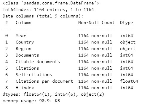
Let's check our data type of each variable by using the following code:

# Return a summary of the DataFrame:
df.info()

Output:

Preparing the Data

From the previous output, we can notice that some variables (column names) contains different data type (Dtype) from others. For instance, The variable "Year" contains integer (int64) data type, whereas "Country" and "Region" contain object data type. Sometimes, we need to use some variables as categorical type so that we do not want Python to make calculations on them, we want to use them as classifiers or factors for other data variables.

In our case, we need "Year, Country and Region" to be a categorical variables (holding categorical data type). We can simply use astype() method as shown in the following code:

# Convert the variables Dtype to categorical:
df["Year"] = df["Year"].astype('category')
df["Country"] = df["Country"].astype('category')
df["Region"] = df["Region"].astype('category')

# Check variables Dtype:
df.info()

Output:

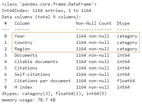
The output above shows that the 3 variables are successfully converted to Categorical Dtype.

Note: In most cases, the data we collect for research or business purposes need more preparing and cleaning process before analyzing and getting insights. The Data preparation and cleaning process will be explained in separate article(s).

Analyzing & Visualizing the Data

In the "Defining the Questions" section, we mentioned that in any data analysis process, we need to define the questions that we need to answer through data analysis. Remember that we are going to analyze the data to answer the following questions:

• What is the total number of publications by year (2017-2021)?

• What are the top regions in number of publications?

• What are the top 5 countries in number of publications?

• How strong the correlation between number of publications and H-index?

1. What is the total number of publications by year (2017-2021)?

We can answer this question by running the following code:

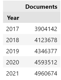
# Group the data by year:
pub_by_year = df[["Year","Documents"]].groupby(["Year"])

# Return the sum of grouped data: 
sum_pub = pub_by_year.sum()
sum_pub

Output:

We can also visualize the results by running the following Seaborn code:

# Visualize data using bar plot:
sns.set_theme(style='darkgrid', font='Calibri', font_scale=1.3)
sns.barplot(data = df, x = "Year", y = "Documents", ci=None)

Output:

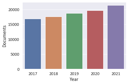
The results above showed that the number of publications increased annually (2017-2021) in which the number of publications in 2021 reached 4,960,674 comparing to 3,904,142 in 2017.

Note: You can do further analysis to know if there is a significant difference in number of publications between years. This can be done using Analysis of Variance(ANOVA) and Post Hoc tests.

2. What are the top regions in number of publications?

We can answer this question by running the following code:

# Group data by region:
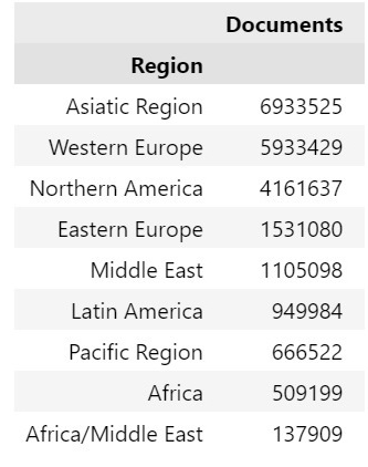
df_by_region = df[[ "Region", "Documents"]].groupby("Region")

# Sort the grouped data:
sorted_by_region = df_by_region.sum().sort_values(by='Documents', ascending=False)

# Return the results:
sorted_by_region

Output:

We can visualize the above table using the following code:

# Visualize data using horizontal bar plot:
sns.set_theme(style='darkgrid', font='Calibri', font_scale=1.3)
sns.barplot(data = df, x="Documents", y="Region", ci=None)

Output:

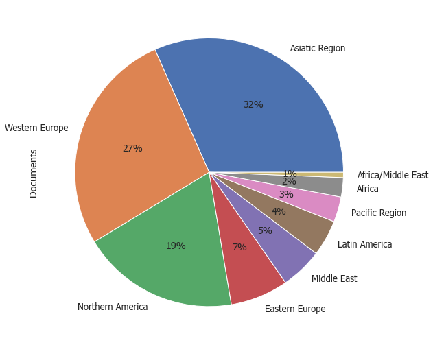
From the results above, it can be noticed that the regions with highest number of publications (From 2017 to 2021) are Asiatic Region, Western Europe, and North America respectively, whereas the lowest was noticed by Africa/Middle East.

3. What are the top 5 countries in number of publications?

We can answer this question by running the following code:

# Group data by country:
pub_countries = df[["Country", "Documents"]].groupby("Country")

# Sort the grouped data:
sort_countries = pub_countries.sum().sort_values(by='Documents', ascending=False)

# Return the first 5 highest values:
top_five= sort_countries.head(5)

top_five

Output:

We can also visualize the results by running the following code:

# Visualizing data using Pandas bar plot:
sns.set_theme(style='darkgrid', font='sans-serif', font_scale=1.3)
top_five["Documents"].plot.barh()

Output:

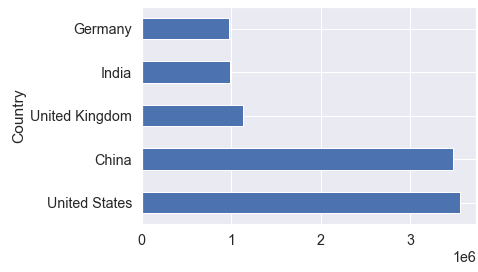
From the results above, it can be noticed that the highest number of publications (From 2017 to 2021) was respectively produced by USA and China followed UK, Germany and India.

4. How strong the correlation between number of publications and H-index?

This questions asks us to find the linear correlation between two variables (Documents and H-index). let's show the data of the two variables using the following code:

cols = ["Documents", "H index"]
df[cols].head(6)

Output:

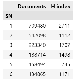
As we previously mentioned, the Documents variable contains the number of publications, whereas the H-index is a metric used to measure the publications impact which is calculated based on the total number of publications and the total number of citations of those publications.

The correlation is simply measures how strong a relationship is between variables. This measure helps us to answer the following question:

"As the number of publications increases, does the H-index increase or decrease?"

To answer this question with Python, we need to run the following code:

# Calculate correlation coefficient and p-value between two variables
corr = pearsonr(df['Documents'], df['Citations'])

# Return the results:
print(corr)

Output:

(0.7320971461581508, 5.883854751333702e-196)

The output above showed two values; the correlation coefficient (r) which is 0.732... and the p-value which is 5.883...e-169.

The correlation coefficient (r) value always ranges between -1 and 1. The closer the r is to +1, the stronger the linear relationship between the two variables; this means as the first variable increases the second one increases as well. On the other hand, the closer the r is to -1, the weaker the relationship between the two variables; this means as the first variable increases, the second one decreases.

Since our r value (0.732) is close to +1 (above 0.70), the variables are highly positively correlated, meaning that the H-index tends to increase linearly as number of publications increases.

The p-value tells us if this relationship (r value) is statistically significant or not. Since our p-value is very small (less than 0.05), the correlation between the two variables are highly significant.

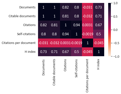
You can also visualize the correlation matrix between all data variables as a heatmap using the following code:

# Corr matrix heatmap:
sns.heatmap(df.corr(), vmin=-1, vmax=1,
annot=True, cmap="rocket_r")

Output:

Conclusions

In this article, we analyzed and visualized SCImago Country Rank data using Python. The SCImago Journal & Country Rank (SJR) is a publicly available portal that includes the journals and country scientific indicators, including number of scientific publications, number of citations and H-index, developed from the information contained in the Scopus database.

The data analysis results indicated that the number of publications increased annually (2017-2021) in which the highest numbers of publications was produced in 2021. The results also showed that the regions with highest number of publications are Asiatic Region, Western Europe, and North America respectively. In addition, the countries produced the highest number of publications was by USA and China respectively followed UK, Germany and India.

The data analysis results also pointed out that a strong positive correlation between the number of publication and the H-index indicating that increased number of publications accompanied by an increase in the publications impact.

References

• Nelli, F. (2015). Python data analytics: Data analysis and science using PANDAs, Matplotlib and the Python Programming Language: Apress.

• Matthes, E. (2019). Python crash course: A hands-on, project-based introduction to programming: no starch press.

• McKinney, W. (2013). Python for data analysis: Agile tools for real-world data (1st ed.). USA: O'Reilly.

• SCImago (2022), (n.d.). SJR — SCImago Journal & Country Rank. Retrieved October 1, 2022, from http://www.scimagojr.com

• J. D. Hunter, "Matplotlib: A 2D Graphics Environment", Computing in Science & Engineering, vol. 9, no. 3, pp. 90-95, 2007.

• Data structures for statistical computing in python, McKinney, Proceedings of the 9th Python in Science Conference, Volume 445, 2010.

• Harris, C.R., Millman, K.J., van der Walt, S.J. et al. (2020). Array programming with NumPy. Nature 585, 357–362. DOI: 10.1038/s41586-020-2649-2.

• Virtanen P. et al. (2020) SciPy 1.0: Fundamental Algorithms for Scientific Computing in Python. Nature Methods, 17(3), 261-272.